Decision Making Under Uncertainty
Alien Defense Radar

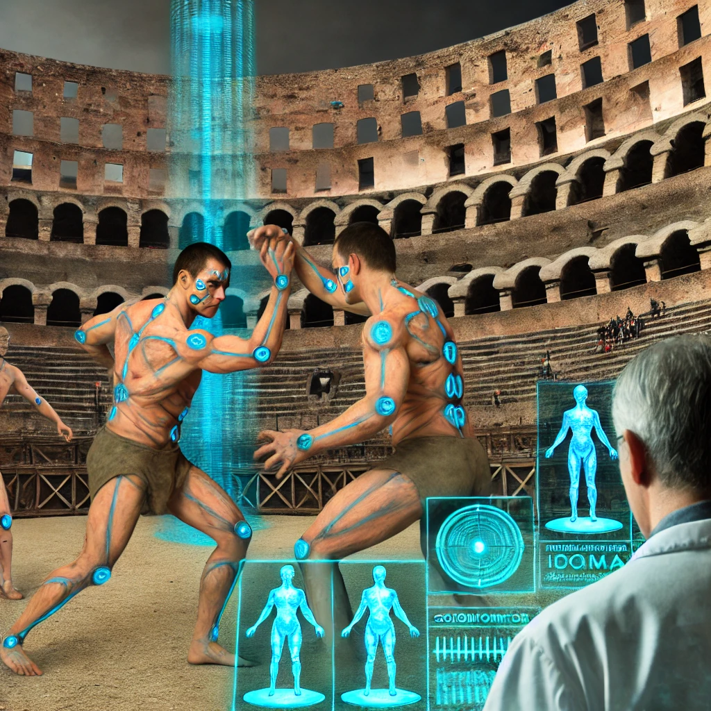
Cybernetic Gladiator Enhancements
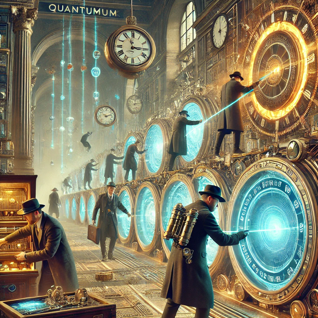
Time-Travel Heist
Introduction
There’s a common theme of uncertainty across these stories. You have to make decisions carefully, balancing between exploration and exploitation. Sure, you could naively sample the space of possible solutions and slowly progress towards the most promising one, but there’s a cost. You’ll either run out of time, money, or patience. There’s a better way.
Enter Bayes’ Theorem.
This post will give you a practical framework for utilizing the Thompson Sampling technique, leveraging Bayesian methods. You’ll be able to solve each of the presented scenarios, and moreover, apply it to mundane cases like A/B testing, dynamic pricing, inventory management, and more.
We’ll focus on high-level ideas and practical frameworks. There are plenty of resources out there for the fine-grained math details. Finally, check out the Google Colab notebook with all the code and simulations.
Background
It all starts with the “criminal” side of Reinforcement Learning (RL) - the multi-armed bandit (MAB) problem, a classic framework in RL that models decision-making under uncertainty.
Imagine an agent choosing between multiple options (the “arms” of slot machines), each providing random rewards from unknown probability distributions. The agent’s goal is to maximize cumulative reward over time by balancing exploration (trying out different arms to learn their reward patterns) and exploitation (leveraging known information to select the best-performing arms).
Each anti-alien radar system, implant, or time-machine for the heist is a distinct “arm”. Initially, these will be random guesses, but as time goes on, decisions will lean towards the most promising ones.
This problem encapsulates the fundamental RL trade-off between exploring new actions and exploiting known ones to achieve optimal long-term outcomes.
A popular approach is the Epsilon-Greedy algorithm, where you choose the most promising arm with a probability of $1-\epsilon$ and explore a random arm with a probability of $\epsilon$. This, however, requires you to set the value of $\epsilon$ in advance (needs fine-tuning), maintain each arm’s statistics, and make the switch at the earliest possible point. A slightly more sophisticated approach is the Upper Confidence Bound (UCB), where you choose the most promising arm based on the estimated mean reward plus an exploration bonus proportional to the inverse of the number of times the arm has been tried. This, however, tends to over-explore suboptimal arms (even with poor performance) and is more computationally complex.
Here, however, we’ll focus on Bayesian methods to sample from a probability distribution of the rewards, balancing exploration and exploitation dynamically, making it a suitable candidate even for non-stationary problems.
Get the Algorithm Selection Framework
A one-page decision guide: when to use Thompson Sampling vs UCB vs Epsilon-Greedy, with trade-offs and production considerations.
Two distributions intertwined
A key insight of Thompson Sampling is that you’re effectively dealing with two probability distributions. The first one models the arm performance (which we ultimately want to know), and the second one iteratively models the first one. In Bayesian terms, these are called the “likelihood” and “prior/posterior”, respectively.
Each parameter distribution is defined by a set of parameters $\theta$. We’ll leverage this fact to model and update them accordingly.
Below is a flowchart that illustrates the Thompson Sampling process. It’s broken down into dependent phases:
- Phase 1: Setting the stage, where we choose both the arm’s likelihood and prior/posterior probability distribution families.
- Phase 2: Running the show - updating beliefs by running simulations.
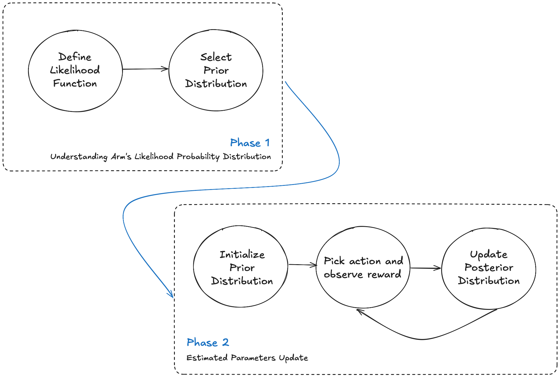
Thompson Sampling Flowchart
Let’s break them down in the context of our stories.
Setting the stage
Alright, let’s dive into the nitty-gritty. The first step in tackling each problem is to identify the nature of each arm’s reward distribution and select the most suitable likelihood probability distribution.
Here’s a cheat sheet for our scenarios:
| Story | Arm | Likelihood Distribution | Parameters | Explanation |
|---|---|---|---|---|
| Alien Invasion | Anti-alien radar system | Bernoulli | $p$ (success probability) | Each test is a hit or miss (binary outcome) |
| Cybernetic Gladiators | Implant | Normal (Gaussian) | $\mu$ (mean), $\sigma$ (standard deviation) | Performance scores likely follow a normal distribution |
| Time-Travel Heist | Timeline | Exponential | $\lambda$ (rate parameter) | Time to complete a heist is always positive and can vary widely |
An example of simulation code simulating the performance of each arm might look like this:
| |
The choice of distribution is crucial — it affects how we update our beliefs and make decisions. Now, knowing each arm’s likelihood distribution and its corresponding parameters, we can pick the most suitable prior distribution.
The prior distribution represents our initial beliefs about the parameters of the likelihood distribution before we have any data. After updating the prior with the data, we get the posterior distribution, which we use for decision-making.
To select a suitable prior distribution, we leverage conjugate priors. These are special prior distributions that are compatible with the likelihood function, resulting in a posterior distribution of the same type as the prior. This makes updating our beliefs a breeze.
Fortunatelly, there are some established conjugate priors for most of the likelihood distributions. To know more, I recommend a good visual breakdown done by John D. Cook.
Here’s a table of likelihood and conjugate prior distribution pairs for each of our stories:
| Likelihood Distribution | Conjugate Prior | Parameters | Explanation |
|---|---|---|---|
| Bernoulli | Beta | $\alpha$ (prior successes), $\beta$ (prior failures) | Beta distribution is suitable for Bernoulli as both deal with probabilities in $[0,1]$. The Beta parameters directly correspond to observed successes and failures, making updates intuitive. |
| Normal (Gaussian) | Normal-Inverse-Gamma | $\mu_0$ (prior mean), $\kappa_0$ (prior sample size), $\alpha_0$, $\beta_0$ (shape and scale) | This joint prior on $(\mu, \sigma^2)$ allows for uncertainty in both mean and variance. It’s conjugate to Normal likelihood and leads to closed-form posterior updates. |
| Exponential | Gamma | $\alpha$ (shape), $\beta$ (rate) | Gamma is conjugate to Exponential and both deal with positive real numbers. The Gamma parameters can be interpreted as prior number of events ($\alpha$) and total time observed ($\beta$), aligning with the Exponential rate parameter. |
Now, having established both distributions, we can start the simulation.
Running the show
We kick things off by initializing the prior distribution parameters. Depending on the information available, this can be done in different ways, but our examples will assume non-informative priors. If you have domain knowledge, use it to speed up convergence.
For a specific number of iterations, we will:
- Sample likelihood parameters $\theta$ from each arm’s prior distribution.
- Select the arm with the highest parameter value $\theta_i$.
- Observe the reward $r$ for the chosen arm.
- Update the arm’s posterior distribution parameters.
- Repeat.
Updating the posterior distribution parameters is the tricky part, as it requires understanding the meaning of each parameter in the prior/posterior distribution. Luckily, the desired formulas can be easily looked up.
In all cases, $n$ is the number of observations and $x_i$ is the observed data. For single-step (online) updates, $n=1$.
| Likelihood-Conjugate Prior Pair | Prior Parameters (Before Data) | Posterior Parameters (After Data) | Notes |
|---|---|---|---|
| Bernoulli - Beta | $\alpha, \beta$ | $\alpha = \alpha + \sum x_i$ $\beta = \beta + n - \sum x_i$ | - $\alpha, \beta$: number of successes and failures respectively |
| Normal (Unknown Mean, Unknown Variance) - Normal Inverse Gamma | $\mu, \lambda, \alpha, \beta$ | $\mu = \frac{\lambda \mu - n \bar{x}}{\lambda + n}$ $\lambda = \lambda + n$ $\alpha = \alpha + \frac{n}{2}$ $\beta = \beta + \frac{1}{2} \sum (x_i - \bar{x})^2 + \frac{\lambda n (\bar{x} - \mu)^2}{2(\lambda + n)}$ | We need toreconstuct the likelihood parameters $\theta = (\mu^{\prime}, \sigma^2)$, therefore: - $\sigma^2 \sim \text{Inverse-Gamma}(\alpha, \beta)$ - $\mu^{\prime} | \sigma^2 \sim N(\mu, \frac{\sigma^2}{\lambda})$ Notice that $\mu^{\prime}$ is sampled from normal distribution, which is conditional on $\sigma^2$. - $\alpha, \beta$: shape and scale parameters Inverse Gamma - $\mu$ : prior mean of the normal distribution - $\lambda$: a positive real number, which is a precision parameter related to how strongly the mean is believed to be centered around $\mu$ |
| Exponential - Gamma | $\alpha, \beta$ | $\alpha = \alpha + n$ $\beta = \beta + \sum x_i$ | - $\alpha$: number of events that have occurred, - $\beta$: rate at which events occur |
How the stories end?
Alien Defense Radar
Imagine you have five radars at your disposal, each named after a Greek god. Here’s the lowdown on their true detection probabilities:
| Radar Name | True Detection Probability |
|---|---|
| Zeus | 0.07 |
| Hera | 0.70 |
| Poseidon | 0.68 |
| Athena | 0.72 |
| Apollo | 0.65 |
Each radar’s detection probability represents its likelihood of successfully spotting an alien spacecraft. Higher probability means a more effective radar system. But here’s the kicker: these probabilities are unknown to us, and we need to learn them through repeated sampling and updating our beliefs.
The plot above showcases the performance of our Thompson Sampling algorithm. Let’s break it down:
- Initial Exploration: Early on, there’s a lot of variation in radar selection. This is the algorithm’s exploration phase, where it’s gathering intel on each option.
- Convergence: As the number of steps increases, the selections zero in on Athena and Hera. These radars are the top performers, and the algorithm is exploiting this knowledge.
- Occasional Exploration: Even after convergence, the algorithm occasionally tests other radars. This ensures it doesn’t miss any changes in radar performance.
- Improving Average Detection Rate: The red line showing the average detection rate starts low but quickly rises and stabilizes. This indicates our algorithm is learning and improving its selections over time.
- Final Performance: By the end of the simulation, we’re hitting an average detection rate of about 0.7, aligning well with the true probabilities of our best radars (Athena at 0.72 and Hera at 0.70).
Cybernetic Gladiators Enhancements
In our cybernetic gladiator scenario, we have five gladiators, each with performance characterized by a Gaussian distribution:
| Gladiator | True $\mu$ (Mean) | True $\sigma$ (Standard Deviation) |
|---|---|---|
| Titan | 75 | 5 |
| Quicksilver | 78 | 6 |
| Enduro | 72 | 4 |
| Neuron | 76 | 5.5 |
| Flex | 74 | 4.5 |
Our goal is to quickly identify the top-performing gladiator through repeated trials. After conducting 500 fights, the algorithm has zeroed in on the best gladiator.
Key takeaways:
- Convergence: With just 500 fights, the algorithm has successfully identified Quicksilver as the top gladiator. This shows the method’s efficiency in determining the optimal choice quickly.
- Dual Parameter Estimation: The algorithm estimates both the mean ($\mu$) and standard deviation ($\sigma$) for each gladiator’s performance, adding complexity to the problem.
- Confidence Regions: The plot shows confidence regions for each gladiator’s performance estimates (red area). Gladiators selected more often (like Quicksilver) have smaller confidence regions, indicating more precise estimates.
- Accuracy: The estimated means (blue line) are close to the true means for each gladiator (green dotted line), showing our algorithm has accurately learned the true performance characteristics.
It’s worth noting that the additional exploration factor was encoded in the algorithm to give less performing gladiators a better chance to estimate their true performance.
Time-Travel Heist
There are four timelines available to our time-travel heist specialists, each with a different heist time:
| Timeline | Average Heist Time |
|---|---|
| Medieval | 1.5 |
| Renaissance | 2.0 |
| Industrial | 1.0 |
| Modern | 0.5 |
Intuitively, it makes the most sense to rob only in the “Modern” timeline, as it has the shortest heist time. The following plot presents the cumulative average heist time after 350 attempts.
The algorithm quickly converges to selecting the most efficient timeline, with occasional exploration of others.
Let’s plot the density of the heist times for each timeline. Notice that to obtain smooth plots, the number of samples increased to 5000. The plot below shows the overlapping distributions for each timeline. The “Modern” timeline variation is the smallest, indicating the algorithm’s high confidence in its estimation.
Summary
Thompson Sampling is a powerhouse for tackling multi-armed bandit problems, as we’ve seen in our scenarios.
Its key strengths include:
- Efficient exploration-exploitation balance: Quickly converges to optimal choices while still exploring alternatives, without requiring hyperparameter tuning.
- Handles uncertainty well: Effectively estimates both mean and variance of unknown distributions.
- Adaptability: Can adjust to changing environments, making it suitable for non-stationary problems like dynamic pricing or content recommendation.
Take our alien defense scenario, for instance. Thompson Sampling swiftly identified the top radar systems while still occasionally testing others, just like a real defense system would adapt to evolving threats.
However, even superheroes have their kryptonite:
- Computational complexity with many arms or complex priors.
- Sensitivity to prior selection, especially with limited initial data.
- Potential performance degradation in highly non-stationary environments.
Choosing between Thompson Sampling and its alternatives depends on the specifics of your problem:
- Contextual Bandits: Great for personalized recommendations, considering user demographics or browsing history.
- Hierarchical Priors: Perfect for grouped decisions, like optimizing treatments across multiple hospitals.
- Gittins Index: Optimal for certain bandit problems, especially with discounted rewards over time. Could be a game-changer in the time-travel heist scenario if the value of successful heists decreased over time.
- Upper Confidence Bound (UCB): Can converge faster in problems with many arms, potentially useful in large-scale A/B testing.
- Epsilon-Greedy: Simple and effective for scenarios with limited computational resources.
When implementing these methods, keep in mind:
- Problem Formulation and Reward Design: Crucial for aligning the algorithm’s objectives with business goals.
- Interpretability: Thompson Sampling offers intuitive probabilistic interpretations, which is gold for stakeholder communication.
- Theoretical Guarantees: Thompson Sampling provides strong regret bounds, essential for critical applications like medical trials.
- Ease of Implementation: Particularly straightforward for those familiar with Bayesian methods.
In conclusion, while Thompson Sampling is a formidable tool for decision-making under uncertainty, it’s essential to consider your problem’s unique requirements when selecting the most appropriate algorithm. Whether optimizing alien defense systems, enhancing gladiators, or planning time heists, the right choice depends on the specific challenges and constraints at hand.
Get the Code + Decision Framework
Receive the Google Colab notebook with all simulations, plus the algorithm selection guide to help you pick the right approach for your use case.
Resources
- Google Colab notebook with all the code and simulations.